Graphs of bounded width as uniformly automatic classes

Bound a graph’s width — tree-depth, tree-width, clique-width, rank-width — and the whole (infinite) class of such graphs becomes a single uniformly automatic class: one tuple of automata, carrying an advice tape that spells out a decomposition of the member graph. Because elements of the presented structure are sets of vertices, first-order logic over the presentation is genuine monadic second-order logic over the graph — this is Courcelle’s theorem, with the automaton actually built.

The pay-off: an MSO property is compiled once for the entire class, and afterwards every member is decided in time linear in its decomposition. Deciding is cheap, so the examples here are deliberately not tiny.

The signature is the same throughout: Sing(x) (x is a singleton), Subset(x, y), and E(x, y) (the singletons x, y are adjacent).

%matplotlib inline
import matplotlib.pyplot as plt
import networkx as nx

_BLUE, _ORANGE = '#4C72B0', '#DD8452'

def draw(G, prog='neato', color=None, title=None, node_size=650, figsize=(5.6, 4.2)):
    # Draw a graph with a graphviz layout; `color` is a vertex set to highlight.
    pos = nx.nx_pydot.graphviz_layout(G, prog=prog)
    node_color = ([_ORANGE if v in color else _BLUE for v in G.nodes]
                  if color is not None else _BLUE)
    fig, ax = plt.subplots(figsize=figsize)
    nx.draw(G, pos, ax=ax, node_color=node_color, node_size=node_size, width=1.4,
            edgecolors='white', linewidths=1.2, with_labels=True,
            font_color='white', font_size=9)
    if title:
        ax.set_title(title, fontsize=11)
    ax.set_axis_off()
    plt.show()

Bounded tree-depth

TreeDepthClass(d) presents every finite graph whose elimination forest has height \(\le d\). The advice is a DFS traversal of that forest — one letter per vertex, encoding its depth and its adjacency to its ancestors — so the advice alphabet has \(2^d - 1\) letters.

from autstr.graphs import TreeDepthClass, TreeDepthGraph

cls = TreeDepthClass(4)
print('relations:', cls.cls.get_relation_symbols())

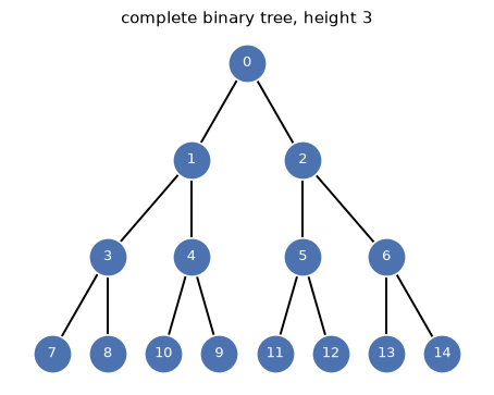
# A complete binary tree of height 3 (15 vertices) has tree-depth exactly 4.
BT = nx.balanced_tree(2, 3)
g = TreeDepthGraph.from_networkx(BT)
print('vertices:', g.num_nodes, ' elimination height:', max(d for d, _ in g.letters))
draw(g.to_networkx(), prog='dot', title='complete binary tree, height 3')

relations: ['U', 'Sing', 'Subset', 'E']
vertices: 15  elimination height: 4

MSO: bipartiteness, compiled once for the whole class

Bipartiteness is there is a set \(c\) so every edge crosses the cut \((c, \bar c)\) — a monadic second-order property. Compiling it yields one automaton over the advice tape; after that each graph is decided by running its advice word.

bipartite = ('exists c.(all x.(all y.((not E(x,y)) or '
             '((Subset(x,c) and (not Subset(y,c))) or '
             '((not Subset(x,c)) and Subset(y,c))))))')

%time bip_dfa, _ = cls.evaluate(bipartite)
print(f'bipartiteness automaton: {bip_dfa.num_states} states\n')

cases = {'complete binary tree': BT,
         'windmill F5 (five triangles)': nx.windmill_graph(5, 3),
         'caterpillar': nx.Graph([(0,1),(1,2),(2,3),(3,4),(0,5),(1,6),(2,7),(3,8),(4,9)])}
for name, G in cases.items():
    print(f'{name:30s} bipartite = {cls.check(bipartite, TreeDepthGraph.from_networkx(G))}')

CPU times: user 467 ms, sys: 17.9 ms, total: 485 ms
Wall time: 485 ms
bipartiteness automaton: 16 states
complete binary tree           bipartite = True
windmill F5 (five triangles)   bipartite = False
caterpillar                    bipartite = True

Extracting a witness 2-colouring

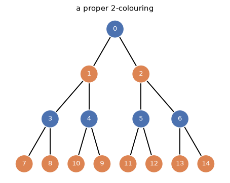
Dropping the outer \(\exists c\) leaves the proper 2-colouring relation with \(c\) free. We take a colouring, verify it with the compiled automaton, and paint it back onto the tree.

coloring = ('all x.(all y.((not E(x,y)) or '
            '((Subset(x,c) and (not Subset(y,c))) or '
            '((not Subset(x,c)) and Subset(y,c)))))')
col_dfa, tapes = cls.evaluate(coloring)

adv = cls.advice(g)
one_side = {v for v, side in nx.bipartite.color(BT).items() if side == 0}
columns = {'advice': adv, 'c': g.encode_set(one_side)}
conv = [tuple(columns[t][i] for t in tapes) for i in range(len(adv))]
print('automaton accepts this colouring:', col_dfa.accepts(conv))
draw(g.to_networkx(), prog='dot', color=one_side, title='a proper 2-colouring')

automaton accepts this colouring: True

Bounded tree-width

TreeWidthClass(w) presents every graph of tree-width \(\le w\); the advice is a tree decomposition. Here the query is connectedness — every non-empty vertex set closed under edges is everything — again compiled once and then run on any member. Width 1 is the forests, on which connectedness is exactly “is a tree”.

from autstr.tree_graphs import TreeWidthClass, TreeWidthGraph

CONNECTED = ('all c.(((exists x.(Sing(x) and Subset(x,c))) and '
             '(all x.(all y.((Subset(x,c) and E(x,y)) -> Subset(y,c))))) '
             '-> (all x.(Sing(x) -> Subset(x,c))))')

tw = TreeWidthClass(1)                     # forests
%time _ = tw.evaluate(CONNECTED)           # one compile for the whole class

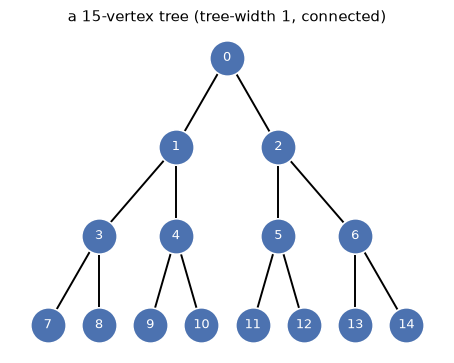
tree = nx.balanced_tree(2, 3)              # a 15-vertex tree: connected
forest = nx.disjoint_union(nx.balanced_tree(2, 2), nx.path_graph(5))   # two components
for name, G in [('balanced tree (15 vertices)', tree), ('tree + path (a forest)', forest)]:
    g = TreeWidthGraph.from_networkx(nx.convert_node_labels_to_integers(G))
    print(f'{name:28s} connected = {tw.check(CONNECTED, g)}')
draw(tree, prog='dot', title='a 15-vertex tree (tree-width 1, connected)')

CPU times: user 477 ms, sys: 3.02 ms, total: 480 ms
Wall time: 480 ms
balanced tree (15 vertices)  connected = True
tree + path (a forest)       connected = False

Bounded clique-width

A \(k\)-expression builds a graph from labelled vertices with disjoint union, relabel, and join (all label-\(i\) to all label-\(j\)). Adjacency is cheap — two vertices are joined exactly when some join node sees them holding its two labels — so MSO queries compile far faster than for tree-width, and the class handles dense graphs.

from autstr.tree_graphs import CliqueWidthClass, CliqueWidthGraph

TWO_COL = ('exists c.(all x.(all y.(E(x,y) -> '
           '(not ((Subset(x,c) and Subset(y,c)) or '
           '((not Subset(x,c)) and (not Subset(y,c))))))))')

cw = CliqueWidthClass(2)
%time two_col, _ = cw.evaluate(TWO_COL)

cases = [('K5', CliqueWidthGraph.clique(5)),
         ('K3,3', CliqueWidthGraph.complete_bipartite(3, 3)),
         ('K4,4', CliqueWidthGraph.complete_bipartite(4, 4))]
for name, G in cases:
    ours, theirs = cw.check(TWO_COL, G), nx.is_bipartite(G.to_networkx())
    assert ours == theirs
    print(f'{name:6s} 2-colourable = {ours}')
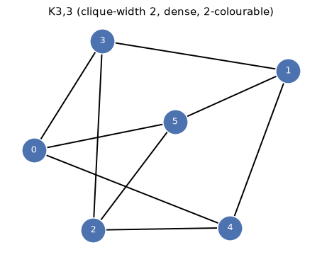
draw(CliqueWidthGraph.complete_bipartite(3, 3).to_networkx(),
     prog='neato', title='K3,3 (clique-width 2, dense, 2-colourable)')

CPU times: user 2.07 s, sys: 20.1 ms, total: 2.09 s
Wall time: 2.1 s
K5     2-colourable = False
K3,3   2-colourable = True
K4,4   2-colourable = True

Bounded rank-width

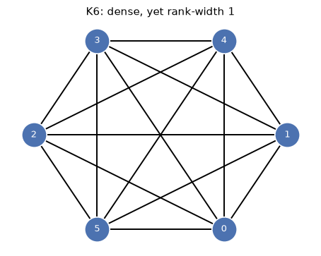
Rank-width bounds the linear-algebraic rank of what crosses each cut of a decomposition. It lower-bounds clique-width but stays bounded on dense graphs — a clique has rank-width 1 — and autstr presents it from the same chain-ring linear algebra as the bounded-rank-width groups. The advice is a rank decomposition annotated with the GF(2) factorisation of its cuts; adjacency is a bilinear form on the vertices’ interface vectors.

from autstr.tree_graphs import RankWidthClass, RankWidthGraph

for build_g, name in [(RankWidthGraph.clique, 'clique K7'),
                      (RankWidthGraph.path, 'path P7'),
                      (RankWidthGraph.cycle, 'cycle C7')]:
    print(f'{name:12s} rank-width = {build_g(7).width}')
print('complete bipartite K3,4 rank-width =', RankWidthGraph.complete_bipartite(3, 4).width)

clique K7    rank-width = 1
path P7      rank-width = 1
cycle C7     rank-width = 2
complete bipartite K3,4 rank-width = 1

# Rank-width-1 members: 2-colourability decided across the class by one automaton.
RW_TWO_COL = ('exists a.(all x.(all y.((not E(x,y)) or '
              '((Subset(x,a) and (not Subset(y,a))) or '
              '(Subset(y,a) and (not Subset(x,a)))))))')
rw = RankWidthClass(1)
for name, G in [('K6 (dense!)', RankWidthGraph.clique(6)),
                ('K3,4', RankWidthGraph.complete_bipartite(3, 4)),
                ('P6', RankWidthGraph.path(6))]:
    print(f'{name:12s} 2-colourable = {rw.check(RW_TWO_COL, G)}')
draw(RankWidthGraph.clique(6).to_networkx(), prog='circo',
     title='K6: dense, yet rank-width 1')

K6 (dense!)  2-colourable = False
K3,4         2-colourable = True
P6           2-colourable = True

# Cycles need rank-width 2; the r=2 class decides their edges implicitly
# (see the implicit-evaluation notebook for why "implicitly").
rw2 = RankWidthClass(2)
C5 = RankWidthGraph.cycle(5)
edges = [(u, v) for u in range(5) for v in range(u + 1, 5)
         if rw2.check_implicit('E(x,y)', C5, x={u}, y={v})]
print('recovered edges of C5:', edges)

recovered edges of C5: [(0, 1), (0, 4), (1, 2), (2, 3), (3, 4)]

---

Every class here is an autstr.uniform (tree-)automatic class: check / evaluate compile and run the query automaton, check_implicit / evaluate_implicit decide the same formulas without building anything — the subject of the implicit-evaluation notebook. The bounded-rank-width group classes share this rank-width machinery and appear in the groups notebook.