Arithmetic and algebra over infinite structures#

Büchi’s and Rabin’s theorems make whole infinite structures computable: encode their elements as finite words (or trees) and recognize the relations with finite automata, and first-order — sometimes monadic second-order — logic becomes decidable by automata operations. autstr turns that theory into code.

This notebook tours the number-theoretic and algebraic structures the library ships with:

Presburger arithmetic \((\mathbb{Z}, +, <)\) — infinite sets as first-class values;
Büchi arithmetic — reasoning about the binary expansions of naturals;
Skolem arithmetic \((\mathbb{N}_{>0}, \cdot)\) — a number as the tree of its prime exponents;
finite Boolean algebras and the localizations \(\mathbb{Z}[1/p]\);
the finite powerset structure MSO0, where first-order logic is Büchi’s MSO.

Groups get their own notebook (groups.ipynb); graphs another (graphs.ipynb).

Variable naming. The formula parser treats a name as a variable only if it matches [a-df-z][0-9]* — a single lowercase letter (never e, which is the parser’s event marker), optionally followed by digits.

Presburger arithmetic over the integers#

\((\mathbb{Z}, +, <)\) is automatic in base 2. autstr.arithmetic exposes it through a small term algebra, so an infinite definable set is an ordinary Python value you can intersect, complement and iterate.

from autstr.arithmetic import VariableETerm as Var
from time import time

x = Var('x')

Infinite sets as first-class values: the Sieve of Eratosthenes#

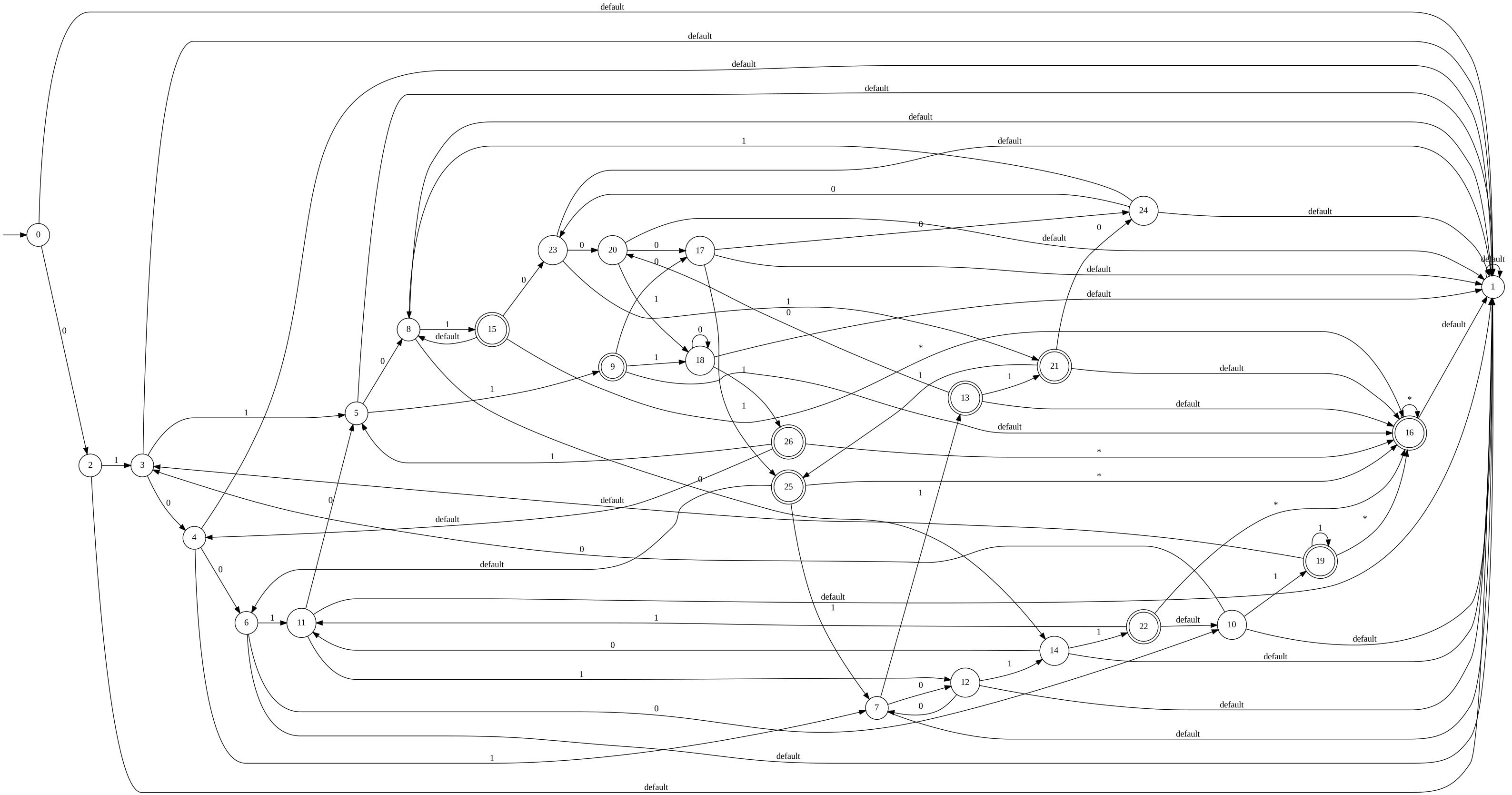
The candidate set starts as the infinite set \(\{2, 3, 4, \dots\}\). Each step reads off its smallest element (elements are enumerated in ascending absolute value) and removes that prime’s proper multiples — a symbolic set difference. The remaining candidates stay an automaton throughout.

def infinite_sieve(steps):
    x = Var('x')
    candidates = (x.gt(1))          # {2, 3, 4, ...}
    primes = []
    for _ in range(steps):
        start = time()
        for p in candidates:        # smallest-first enumeration
            primes.append(p[0])
            break
        print(f"next prime {primes[-1]}  ({time() - start:.3f}s)")
        y = Var('y')
        multiples = (x.eq(primes[-1] * y)).drop('y')
        candidates = candidates & ~multiples
    return primes, candidates

primes, remaining = infinite_sieve(steps=3)
print('primes found:', primes)
remaining.evaluate().show_diagram()

next prime 2  (0.014s)
next prime 3  (0.050s)
next prime 5  (0.111s)
primes found: [2, 3, 5]

../_images/9e1cc01e7021a0dbb8b14b8587bc9f1b1b7f269a2c74752a7a1f68f9d1a1161a.svg

Integer linear systems#

Integer linear systems are NP-hard in general, but they are first-order definable over \((\mathbb{Z}, +)\), so we can build them and read off (or rule out) solutions.

x, y, z = Var('x'), Var('y'), Var('z')

eqn_sys = (x + y).eq(6) & (y + z).eq(12) & (x + z).eq(10)
for s in eqn_sys:
    print('solution:', s)

solution: (2, 4, 8)

unsolvable = (3 * y + 5 * z).eq(1) & (x + y).eq(5) & (10 * z + x).eq(17)
print('has a solution:', not unsolvable.isempty())

has a solution: False

Büchi arithmetic: reasoning about binary expansions#

Büchi arithmetic extends Presburger with \(V_2(x)\) — the largest power of two dividing \(x\) — which is exactly the power to talk about the bits of a number. Many relations are generated on creation, so the first build takes a moment.

from autstr.buildin.presentations import BuechiArithmetic

ba = BuechiArithmetic()
ba.automata['A'].show_diagram()          # the addition relation A(x, y, z): x + y = z

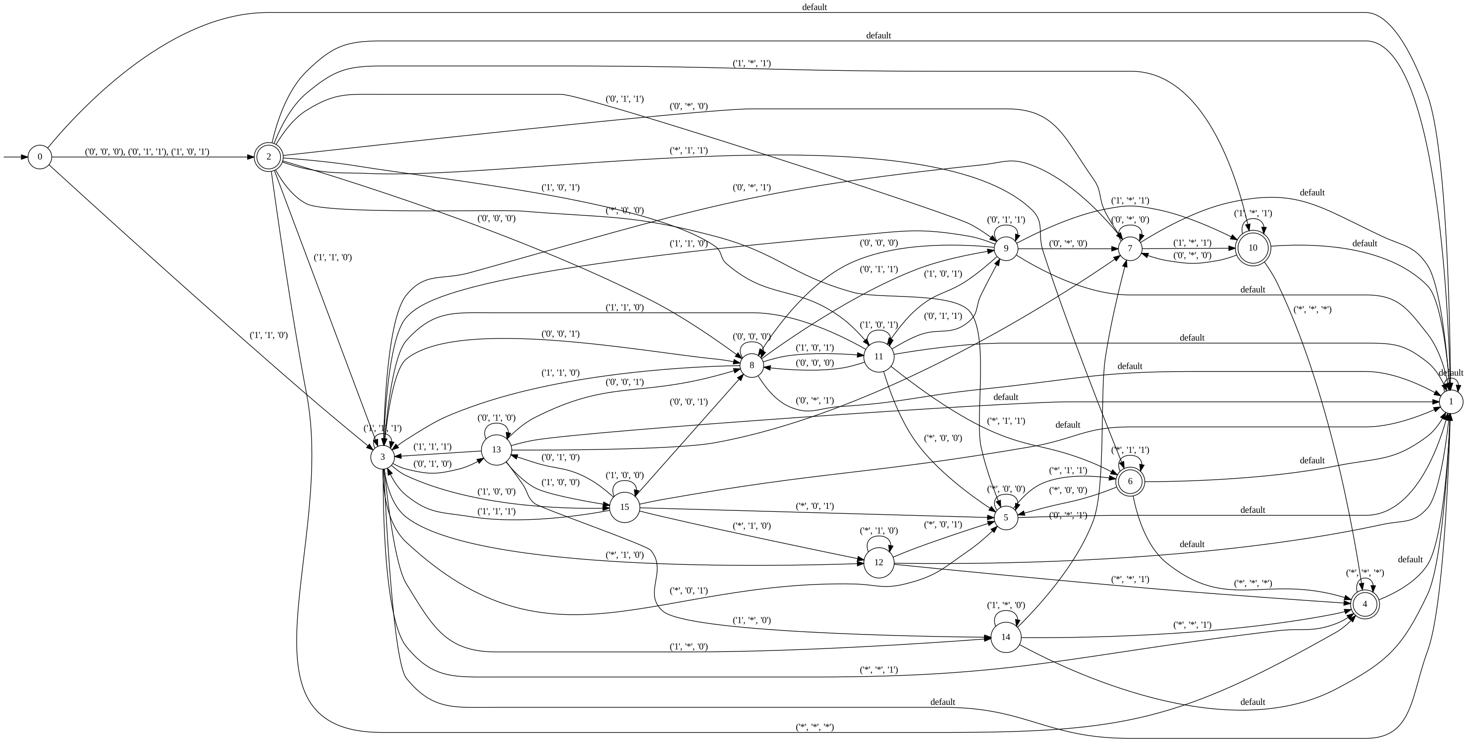
../_images/ba6e09433ba8f4cbc8dad59373ff856c88bf37c86146aee9e5a7205de5f8a0ca.svg

Everything else is defined first-order from addition, the same bootstrap the library uses everywhere. Zero is the unique \(x\) with \(x + x = x\); one is the only other number whose additive decompositions are all trivial; the successor and the powers of two follow.

ba.update(O='A(x,x,x)')                                        # zero
ba.update(I='not O(x) and forall y z.(O(y) or O(z) or not A(y, z, x))')   # one
ba.update(S='exists x.(I(x) and A(u, x, v))')                  # successor S(u, v): v = u + 1
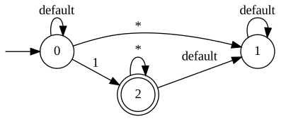
ba.update(P='B(x,x)')                                          # powers of two
ba.update(Smaller='exist z.(not O(z) and A(x, z, y))')         # strict order
ba.automata['P'].show_diagram()

../_images/2d48cb906f265a8c6c7322a1de78f72ed4d54ffdd75e9eb14ae60cb6d88ae782.svg

A small theorem, proved by automaton#

For every positive \(x\) there is a power of two in \([x, 2x]\). A sentence has no free variables, so its automaton is a single state — accepting exactly when the sentence is true.

sandwich = ('forall x.(O(x) or exists y u v w.('
            'A(x, x, y) and A(x, u, v) and P(v) and A(v, w, y)))')
print('sandwich theorem holds:', ba.check(sandwich))

sandwich theorem holds: True

Skolem arithmetic: multiplication as a tree#

\((\mathbb{N}_{>0}, \cdot)\) is not automatic over strings, but it is tree-automatic: write \(n = \prod_i p_i^{e_i}\) as a spine of primes with each exponent hanging off as a binary chain, and multiplication becomes componentwise addition along the branches (Rabin’s theorem, made executable).

from autstr.buildin.tree_presentations import skolem_arithmetic

skolem = skolem_arithmetic()
print('360 = 2^3 * 3^2 * 5 round-trips to:', skolem.decode(skolem.encode(360)))

M = skolem.evaluate('M(x,y,z)')                 # one automaton, an infinite domain
enc = skolem.encode
for a, b, c in [(6, 10, 60), (7, 13, 91), (6, 11, 65)]:
    print(f'{a} * {b} = {c}?  {M.accepts(enc(a), enc(b), enc(c))}')

= 2^3 * 3^2 * 5 round-trips to: 360
* 10 = 60?  True
* 13 = 91?  True
* 11 = 65?  False

# Divisibility is first-order over multiplication alone:  x | y  iff  exists z. x*z = y
divides = skolem.evaluate('exists z.(M(x,z,y))')
for a, b in [(3, 12), (5, 12), (7, 91)]:
    print(f'{a} divides {b}: {divides.accepts(enc(a), enc(b))}')

divides 12: True
divides 12: False
divides 91: True

Finite Boolean algebras#

autstr.algebra presents whole families of finite structures as one uniformly automatic class: a single tuple of automata carries an extra advice tape, and fixing the advice pins down one member. The Boolean algebra with \(n\) atoms is the advice 1 repeated \(n\) times; elements are bitvectors of length \(n\).

from autstr.algebra import FiniteBooleanAlgebras

bool_alg = FiniteBooleanAlgebras()
n = 4
print('Meet({0,1}, {1,2}) = {1}:', bool_alg.check('Meet(x,y,z)', n, x={0, 1}, y={1, 2}, z={1}))
print('Atom({3}):            ', bool_alg.check('Atom(x)', n, x={3}))

# One compiled automaton decides a property for every size at once.
proper = 'exists x.(exists y.(Compl(x,y) and (not Leq(x,y))))'
dfa, tapes = bool_alg.evaluate(proper)
for size in [0, 1, 5]:
    advice = bool_alg.advice(size)
    print(f'n={size}: has a complemented non-subalgebra element =',
          dfa.accepts([(s,) for s in advice]))

Meet({0,1}, {1,2}) = {1}: True
Atom({3}):             True
n=0: has a complemented non-subalgebra element = False
n=1: has a complemented non-subalgebra element = True
n=5: has a complemented non-subalgebra element = True

The localization \(\mathbb{Z}[1/p]\)#

z1p_localization(p) is a factory: for each prime \(p\) it produces the additive group \(\mathbb{Z}[1/p] = \{\, a/p^k : a \in \mathbb{Z},\ k \ge 0 \,\}\) together with an automatic presentation of \((\mathbb{Z}[1/p], +)\). The encoding interleaves the integer and fractional digits around the radix point so both expansions grow rightward and stay aligned; signed addition A, zero Z and equality Eq are then defined from magnitude addition.

from autstr.algebra import z1p_localization

z2 = z1p_localization(2)
half, three_q = z2.from_fraction(1, 2), z2.from_fraction(3, 4)
print('1/2 + 3/4 = 5/4:', z2.check('A(x,y,z)', x=half, y=three_q, z=z2.add(half, three_q)))
print('encoding of 5/4:', z2.encode(z2.from_fraction(5, 4)))

1/2 + 3/4 = 5/4: True
encoding of 5/4: ['+', '1_0', '0_1']

The first-order theory tells the primes apart#

Every element of \(\mathbb{Z}[1/p]\) is divisible by \(p\) but by no other prime. Both are first-order sentences, so the presentations decide them — and disagree exactly where the primes differ.

z3 = z1p_localization(3)
div2 = 'all x.(exists y.(A(y,y,x)))'                           # 2 | x for all x
div3 = 'all x.(exists y.(exists w.(A(y,y,w) and A(w,y,x))))'   # 3 | x for all x
for name, s in [('Z[1/2]', z2), ('Z[1/3]', z3)]:
    print(f'{name}:  2-divisible={s.check(div2)}   3-divisible={s.check(div3)}')

Z[1/2]:  2-divisible=True   3-divisible=False
Z[1/3]:  2-divisible=False   3-divisible=True

The finite powerset structure MSO0#

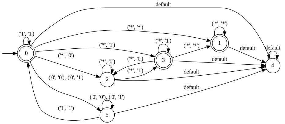
The finite subsets of \(\mathbb{N}\), ordered by \(\subseteq\) with singletons, successor and order on singletons, form the structure MSO0. A finite set is a \(\{0,1\}\)-word (position \(i\) set iff \(i\) is a member), and — by Büchi’s theorem — first-order logic over MSO0 is precisely monadic second-order logic over \((\mathbb{N}, <)\): the definable sets are exactly the regular ones.

from autstr.buildin.presentations import MSO0

mso0 = MSO0()
print('relations:', mso0.get_relation_symbols())
mso0.automata['Subset'].show_diagram()

relations: ['U', 'Subset', 'Sing', 'Succ', 'Lt_sing', 'In', 'Eq_set', 'Leq_sing', 'Gt_sing', 'Min', 'Max', 'Intersect', 'Union', 'SetMinus', 'Geq_sing']

../_images/b9a7e49cbf56c5e825d2a5cd5deab9dda163e343b88be411618dfe78c541c0ef.svg

# Self-contained MSO sentences, each decided by a one-state automaton.
print('there is a singleton:               ', mso0.check('exists x.(Sing(x))'))
print('every singleton has a successor:    ',
      mso0.check('all x.((not Sing(x)) or exists y.(Succ(x,y)))'))
print('there is a least singleton:         ',
      mso0.check('exists x.(Sing(x) and all y.((not Sing(y)) or Leq_sing(x,y)))'))

there is a singleton:                True
every singleton has a successor:     True
there is a least singleton:          True

Every family above is an instance of autstr.uniform.UniformlyAutomaticClass (or its tree analog), whose define() turns first-order definitions over small primitive automata into new relations — the uniform version of the Büchi-arithmetic bootstrap. The groups and graphs notebooks push the same machinery to non-abelian groups and to graphs of bounded width.

Arithmetic and algebra over infinite structures

Contents